Example · 03

Write an inverse simulation

This example uses YASPS at its lowest public layer. We construct the Hessian, jacobians, and gradient ourselves, call a solver directly, and construct the adjoint method ourselves.

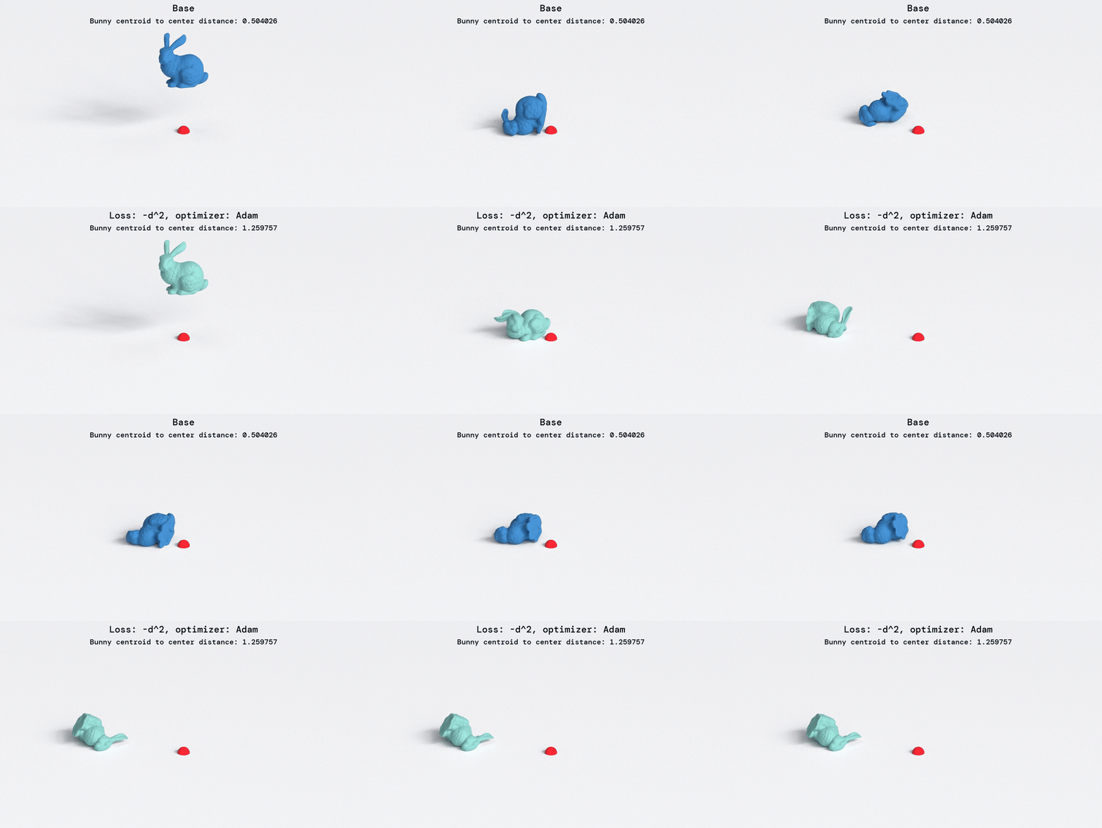
A bunny trajectory changing as its tetrahedron materials are optimized — The original and optimized trajectories. Each optimization round runs the simulation forward and then replays it backward.

This tutorial follows YASPS’s bunny_material_optimization_surface_motion_away_from_origin example. We focus on its two per-tetrahedron material fields.

We will not rebuild the mesh, collision primitives, CCD object, or forward Newton loop here. Use the dropping example for those pieces. This example begins with a working forward simulation and concentrates on what has not appeared before.

Start from a forward simulation

Our forward state is the bunny’s current vertex position. Because implicit Euler uses velocity from two saved positions, a frame depends on both last_position and last_last_position:

import numpy as np
from yasps import attribute, differentiator, solver, vector
from helpers import inertia, stable_neo_hookean

velocity = (last_position - last_last_position) / dt
inertia_energy = vertices.addAttribute("inertia_energy", computed_attribute=inertia(last_position, velocity, dt, position, mass))

The following objects are assumed to exist from the forward setup:

Name	Meaning
`position`	live `3 × 1` vertex position minimized each frame
`last_position`	position at the start of the current frame
`last_last_position`	position at the start of the previous frame
`elastic_energy`	stable Neo-Hookean energy on tetrahedra
`inertia_energy`	implicit-Euler inertia on vertices
`collision_energies`	dynamic point–point, point–edge, point–triangle, and edge–edge energies
`friction_energies`	matching dynamic friction energies

collision_energies and friction_energies are ordinary Python lists containing the computed energy attributes created by the forward simulation:

collision_energies = [pp_energy, pe_energy, pt_energy, ee_energy]
friction_energies = [pp_friction_energy, pe_friction_energy, pt_friction_energy, ee_friction_energy]

The forward scene still registers these energies and minimizes only position, exactly as in the first example.

Put the design on the tetrahedra

The inverse problem changes the material distribution, not the rest shape. Create one Young’s modulus and one Poisson ratio for every tetrahedron:

tet_indices = np.asarray([...], dtype=np.uint32).reshape((-1, 4))
num_tets = len(tet_indices)
tets = bunny.addPrimitive("tets", numInstances=num_tets)
young = tets.addConstant("young")
poisson = tets.addConstant("poisson")

young and poisson each contain num_tets values. Initialize the fields and form the Lamé parameters used by the elastic expression:

young_values = np.full(num_tets, 15_259.25455816859)
poisson_values = np.full(num_tets, 0.3045697005781997)
young.updateValue(young_values)
poisson.updateValue(poisson_values)
mu = young / (2.0 * (1.0 + poisson))
lam = young * poisson / ((1.0 + poisson) * (1.0 - 2.0 * poisson))
elastic_energy = tets.addAttribute("elastic_energy", computed_attribute=stable_neo_hookean(tet_rest_positions, tet_positions, mu, lam, dt))

They are constants in the forward solve because position is the only forward unknown. We can still explicitly differentiate an energy with respect to a constant in the inverse pass.

Define the objective

We want the final bunny to move away from the origin. Minimizing the negative squared distance produces that behavior:

away_weight = simulation.addConstant("away_weight")
away_weight.updateValue(10.0)
offset = position - attribute.to_array([0.0, 0.0, 0.0], rows=3, cols=1)
away_loss = vertices.addAttribute("away_loss", computed_attribute=-away_weight * offset.dot(offset))

The loss is not a forward energy. Registering it with the scene would make the physical simulation push the bunny away from the origin. Instead, differentiate it separately so it becomes the terminal right-hand side of the inverse problem:

loss_gradient = differentiator().diff1([away_loss], [position])

diff1 returns a gradient because away_loss is scalar.

Differentiate the equilibrium equation

At the converged state of one frame, the forward energy should satisfy

g(position, last_position, last_last_position, young, poisson) = 0.

In simpler words, the gradient should be 0 at converged frame.

Differentiating this equation gives the matrices needed by the reverse pass:

Object	Derivative	Purpose
state hessian `H`	`∂g / ∂position`	solve for the adjoint variable
previous-state jacobian `B`	`∂g / ∂last_position`	propagate to the previous frame
older-state jacobian `D`	`∂g / ∂last_last_position`	propagate through velocity to one more frame back
material jacobian `C`	`∂g / ∂young` or `∂g / ∂poisson`	convert the adjoint into a material gradient

These are second derivatives of scalar energy terms, so we construct all four kinds with differentiator.diff2.

Construct the state hessian

Differentiate each forward energy separately because their projection and dynamic-instance settings differ:

elastic_hessian = differentiator().diff2([elastic_energy], [position], [position], projection_method=1)
inertia_hessian = differentiator().diff2([inertia_energy], [position], [position], projection_method=-1)
collision_hessians = [differentiator().diff2([energy], [position], [position], projection_method=2, dynamic_instances=True) for energy in collision_energies]
friction_hessians = [differentiator().diff2([energy], [position], [position], projection_method=2, dynamic_instances=True) for energy in friction_energies]

When the two target lists match, diff2 returns a hessian. We use the same projection methods as the forward Newton solve, which gives a projected approximate adjoint system that can be solved by YASPS’s positive-semidefinite solver.

Hessians with the same target layout can be added before numeric assembly:

adjoint_hessian = elastic_hessian + inertia_hessian
for energy_hessian in collision_hessians + friction_hessians:
  adjoint_hessian = adjoint_hessian + energy_hessian

At this point adjoint_hessian stores symbolic assembly work. Its numerical values are produced later, after we restore a particular frame.

Construct the state jacobians

The next state depends on last_position through inertia and friction, so build those mixed derivatives and add them:

previous_position_jacobian = differentiator().diff2([inertia_energy], [position], [last_position])
for energy in friction_energies:
  previous_position_jacobian = previous_position_jacobian + differentiator().diff2([energy], [position], [last_position], dynamic_instances=True)

Only inertia depends on last_last_position in this example:

previous_previous_position_jacobian = differentiator().diff2([inertia_energy], [position], [last_last_position])

Because the two target lists differ, these calls return rectangular jacobian objects. Their row layout follows position; their column layout follows the relevant historical state.

Construct the material jacobians

Now differentiate the elastic residual with respect to the two per-tetrahedron fields:

young_jacobian = differentiator().diff2([elastic_energy], [position], [young])
poisson_jacobian = differentiator().diff2([elastic_energy], [position], [poisson])

For n vertices and m tetrahedra, each material jacobian has 3n rows and m columns. A transpose multiplication will therefore turn a vertex-sized adjoint vector into one scalar gradient per tetrahedron.

Save the complete forward trajectory

The reverse pass must evaluate every derivative at the exact state used by the forward solve. Save the converged positions and both kinds of dynamic pair topology:

trajectory = {
  "positions": [position.value.get().copy()],
  "collision_pairs": [],
  "friction_pairs": [],
}

for frame in range(NUM_FRAMES):
  solve_one_forward_frame()
  trajectory["positions"].append(position.value.get().copy())
  trajectory["collision_pairs"].append(save_collision_pairs())
  trajectory["friction_pairs"].append(save_friction_pairs())

Here we save not only the positions attribute’s values at convergence, but also the collision pairs so that the reverse pass can reconstruct the dynamic pair topology, as well as the correct Hessian and jacobian matrices.

Assemble and solve one adjoint system

Create a solver directly rather using the scene class or the minimizer class:

adjoint_solver = solver()

After restoring a frame, assemble the numeric hessian using the current attribute values and current dynamic connectivity:

# restore the values at the converged state
position.updateValue(...)
# restore the collision connectivity
pp2v.updateConnectivity(...)
...
# recompute the adjoint hessian's numeric value
adjoint_hessian.compute()

Now solve H μ = λ, where λ is the state gradient already accumulated for this frame:

error_code = adjoint_solver.computeSolution(adjoint_hessian, state_gradient, None, tolerance=1e-8, maxIterations=20_000, zero_initial_guess=True)
if error_code < 0:
  raise RuntimeError(f"adjoint solve failed with error code {error_code}")

auxiliary = vector(state_gradient.size)
auxiliary.updateValue(adjoint_solver.solution)

adjoint_solver.solution is the device-resident μ. We copy it into a YASPS vector because the sparse matrix multiplication API consumes compatible vectors.

Apply jacobians with transpose SpMV

Here we once again, use the saved values to recompute the jacobian matrices, then perform an spmv with transpose=True:

previous_position_jacobian.compute()
previous_contribution = previous_position_jacobian.spmv(auxiliary, transpose=True)

previous_previous_position_jacobian.compute()
previous_previous_contribution = previous_previous_position_jacobian.spmv(auxiliary, transpose=True)

young_jacobian.compute()
young_contribution = young_jacobian.spmv(auxiliary, transpose=True)

poisson_jacobian.compute()
poisson_contribution = poisson_jacobian.spmv(auxiliary, transpose=True)

The operations are Bᵀμ, Dᵀμ, C_youngᵀμ, and C_poissonᵀμ. They return vectors with exactly the sizes needed by the previous states and material fields.

Replay the simulation backward

Let’s first create some variables for storing and accumulating the adjoint gradients:

position_adjoints = [vector(loss_gradient.size) for _ in range(NUM_FRAMES + 2)]
young_gradient = vector(young_jacobian.cols)
poisson_gradient = vector(poisson_jacobian.cols)

The loss is evaluated only at the final state. Let’s first compute it:

position.updateValue(trajectory["positions"][-1])
loss_gradient.compute()
position_adjoints[-1].updateValue(loss_gradient)

Now walk backward. Each iteration restores one converged forward frame, solves one adjoint system, propagates to the two earlier states, and accumulates the two per-tetrahedron gradients:

for frame in range(NUM_FRAMES - 1, -1, -1):
  position.updateValue(trajectory["positions"][frame + 1])
  last_position.updateValue(trajectory["positions"][frame])
  last_last_position.updateValue(trajectory["positions"][max(0, frame - 1)])
  restore_collision_pairs(trajectory["collision_pairs"][frame])
  restore_friction_pairs(trajectory["friction_pairs"][frame])

  adjoint_hessian.compute()
  error_code = adjoint_solver.computeSolution(adjoint_hessian, position_adjoints[frame + 2], None, tolerance=1e-8, maxIterations=20_000, zero_initial_guess=True)
  if error_code < 0:
    raise RuntimeError(f"adjoint solve failed with error code {error_code}")

  auxiliary = vector(position_adjoints[frame + 2].size)
  auxiliary.updateValue(adjoint_solver.solution)

  previous_position_jacobian.compute()
  previous_previous_position_jacobian.compute()
  young_jacobian.compute()
  poisson_jacobian.compute()

  position_adjoints[frame + 1] = position_adjoints[frame + 1] - previous_position_jacobian.spmv(auxiliary, transpose=True)
  position_adjoints[frame] = position_adjoints[frame] - previous_previous_position_jacobian.spmv(auxiliary, transpose=True)
  young_gradient = young_gradient - young_jacobian.spmv(auxiliary, transpose=True)
  poisson_gradient = poisson_gradient - poisson_jacobian.spmv(auxiliary, transpose=True)

Update the material with Adam

After the adjoint gradient is accumulated, let’s apply an Adam update. This helper also clips the physical parameters to a valid range:

def adam_update(values, gradient, first_moment, second_moment, step, learning_rate, lower, upper):
  first_moment = 0.9 * first_moment + 0.1 * gradient
  second_moment = 0.999 * second_moment + 0.001 * gradient * gradient
  corrected_first = first_moment / (1.0 - 0.9 ** step)
  corrected_second = second_moment / (1.0 - 0.999 ** step)
  updated = values - learning_rate * corrected_first / (np.sqrt(corrected_second) + 1e-8)
  return np.clip(updated, lower, upper), first_moment, second_moment

Create one pair of moment buffers for each design field:

young_first = np.zeros(num_tets)
young_second = np.zeros(num_tets)
poisson_first = np.zeros(num_tets)
poisson_second = np.zeros(num_tets)

After each backward replay, update the physical values and send them back to their YASPS constants:

young_values, young_first, young_second = adam_update(young_values, young_gradient.value.get(), young_first, young_second, step, 0.8, 500.0, 500_000.0)
poisson_values, poisson_first, poisson_second = adam_update(poisson_values, poisson_gradient.value.get(), poisson_first, poisson_second, step, 0.8, 0.1, 0.49)
young.updateValue(young_values)
poisson.updateValue(poisson_values)

Run the optimization

One optimization round is now:

for step in range(1, NUM_ADAM_STEPS + 1):
  reset_forward_state()
  trajectory = run_forward_trajectory()
  young_gradient_values, poisson_gradient_values = run_backward_trajectory(trajectory)
  young_values, young_first, young_second = adam_update(young_values, young_gradient_values, young_first, young_second, step, 0.8, 500.0, 500_000.0)
  poisson_values, poisson_first, poisson_second = adam_update(poisson_values, poisson_gradient_values, poisson_first, poisson_second, step, 0.8, 0.1, 0.49)
  young.updateValue(young_values)
  poisson.updateValue(poisson_values)

run_forward_trajectory() contains the high-level scene loop from example 1. run_backward_trajectory() contains the explicit hessian assembly, direct solver call, and transpose SpMV loop developed above.